How to Create Excel Column Names
Our guide continues below with additional information to answer the question of how do you name columns in Excel, including pictures of these steps. Putting descriptions for columns at the top of your spreadsheet is a great way to label your data and make it easier to understand. This is such a common practice that Excel actually gives a name to it, which is the “title row.” You can even choose to freeze that title row if you would like it to remain visible when you scroll down your spreadsheet. Our tutorial below will show you how to insert a new row at the top of your spreadsheet so that you can use it as a title row. We will also discuss how to turn a selection with title rows into a table in Excel so that you can perform other actions on your data, such as filtering and sorting. Check out our Microsoft Excel add column tutorial and learn about easy ways to get sums of cell data.
How to Add a Title Row to a Spreadsheet in Excel 2013 (guide with Pictures)
The steps in this article were performed in Microsoft Excel 2013. These steps will work in other versions of Excel as well. We will also discuss turning a selection of cells into a table in Excel in the section below, which may be closer to the result you are trying to achieve, if adding the title row isn’t the desired result.
Step 1: Open your spreadsheet in Excel 2013.
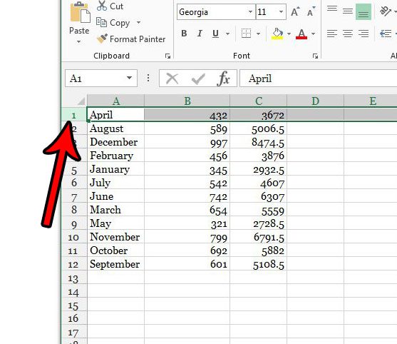
Step 2: Click the top row number at the left side of the spreadsheet.
If you haven’t hidden any rows, then this should be row 1.
Step 3: Right-click the selected row number, then choose the Insert option.
You can also insert a new row when a row is selected by pressing Ctrl + Shift + + on your keyboard.
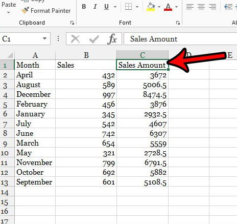
Step 4: Add column names into the blank cells in this new row.
Our article continues below with another answer to the question of “how do you name columns in Excel” which involves creating a table from your existing data.
How to Turn a Selection Into a Table in Excel 2013
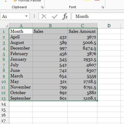
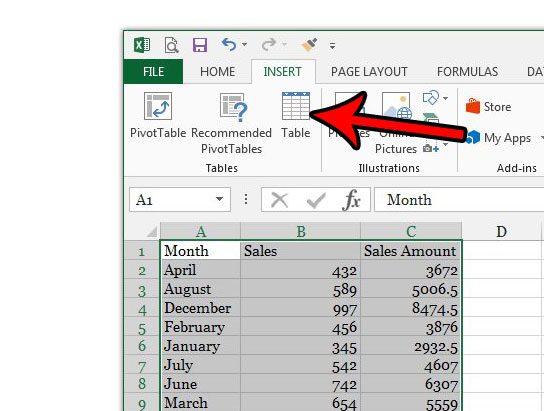
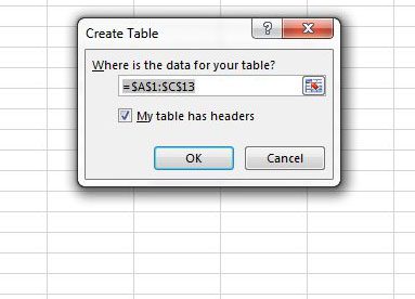
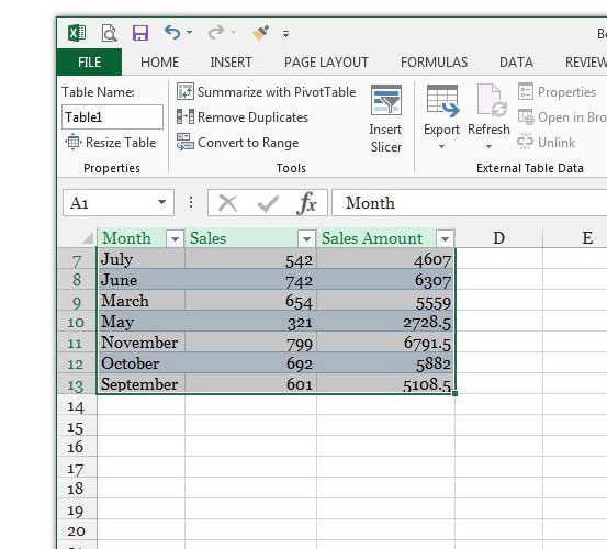
Now that you’ve added your column names, you can go one step further by turning a selection into a table with the steps below. For more information, you can read our complete guide to creating tables in Excel. Step 1: Select the cells that you want to include in the table. Step 2: Click the Insert tab at the top of the window. Step 3: Select the Table button in the Tables section of the ribbon. Step 4: Confirm that the My table has headers option is checked, then click the OK button. If you scroll down in your table you will see that the table column names replace the column letters while the table is still visible. Hopefully this has helped you to answer the question of how do you name columns in Excel? Now that you’ve set up your table in the manner that you want, one of the next hurdles will be getting it to print properly. Check out our Excel printing guide for some tips on making your spreadsheet a little easier to manage when it’s printed on paper.
Additional Sources
After receiving his Bachelor’s and Master’s degrees in Computer Science he spent several years working in IT management for small businesses. However, he now works full time writing content online and creating websites. His main writing topics include iPhones, Microsoft Office, Google Apps, Android, and Photoshop, but he has also written about many other tech topics as well. Read his full bio here.
You may opt out at any time. Read our Privacy Policy