The steps in this article are going to show you where to find the display options and print options that control the gridlines in your spreadsheet. You can then adjust these settings to add gridlines in Excel 2016 in whatever capacity you require. Microsoft Excel has been the industry standard for spreadsheets for a very long time. However, anyone that has tried to print a spreadsheet in Excel has likely found that the default settings won’t include gridlines when you print your data. Luckily you can format cells in a variety of ways in Excel, and one of those options lets you control whether or not gridlines are displayed on the screen and on the printed page. Our guide below will show you where to find these settings.
How to Insert Gridlines in Excel 2016
Our article continues below with additional information on how to make gridlines in Excel, including pictures of these steps.
How to Print or View Gridlines in Excel 2016 (Guide with Pictures)
The steps in this tutorial were performed in the Microsoft Excel for Office 365 version of the application, but will also work in most other versions of Excel, such as Excel 2010, Excel 2013, or Excel 2016.
Step 1: Open the file where you wish to view or print the gridlines.
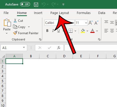
Step 2: Click the Page Layout tab at the top of the screen.
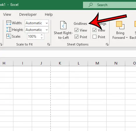
Step 3: Locate the Gridlines section in the Sheet Options group of the ribbon, then click the check box to the left of each option you wish to enable.
You can do a print check before actually making a physical copy of your spreadsheet by going to File > Print and looking at the data in the Print Preview window at the right side of the window. You will be able to see whether or not the gridlines are going to print by looking there. If you would like to remove gridlines, click the box to the left of whichever option you wish to modify to remove the checkmark.
More Information on How to Add Gridlines in Excel 2016
Excel does not give you a way to change the gridline color from the ribbon, but you can change the color of the gridlines through the Excel Options menu. Click the File tab at the top-left of the window, then click the Options button at the bottom of the left column. Choose the Advanced tab at the left of that window, then scroll down to the Display options for this worksheet section. Click the button to the right of Gridline color, then choose the desired color. Click the OK button to close the dialog box and save your changes.
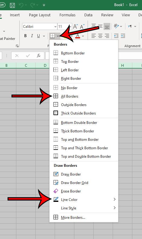
You do have another option which can provide something similar to gridlines, called Borders. First, select all of the cells for which you wish to apply a border. Then, click the Home tab at the top of the window and find the Font section of the ribbon. Next you can click the arrow to the right of the Borders button and choose the All Borders option. You can then open that menu again and select the Line Color option to set the desired color for the borders, which will give you a different border color or gridline color.
Rather than navigating to the Borders option on the Home tab, you can also right-click on your selected cells and access the Borders menu from there. The menu accessible through the right-click option includes things like Fill Color, too, which you may need to adjust if you want no fill color in your cells, but one is currently set.
There is also an option on the View tab which can let you show gridlines or hide them as well. However, adjusting this option won’t affect whether or not your gridlines print.Electing to print gridlines in your Excel spreadsheet is just one of many print settings that can improve the way your data looks on the printed page. Some other options can be found on the Print menu, accessible on the File tab. For example, if you click the No Scaling button at the bottom of that menu you have the option to fir all of your columns, all of your rows, or even your entire worksheet on one page.While your Excel worksheet will often be easier to read on the page or view on the screen when Excel gridlines are visible, you may encounter some scenarios where you would prefer to hide gridlines instead. Luckily this can be accomplished by simply going back to the Page Layout tab and click the gridlines check box for whichever option you would like to hide or disable. You can remove gridlines or add gridlines whenever you want without affecting any of your data.MS Excel cell borders exist on top of the gridlines, so they can add some confusion. Additionally, the cell background color also overrides any gridline display. If you aren’t seeing your gridlines but you have enabled them, it’s a good idea to go to the Font group section on the Home tab and adjust border settings or remove fill color if you don’t see your gridlines. Note that a white fill color is different than the No Fill option.
Google Sheets also allows you to control the display and printing of your gridlines. Thi setting is found in Google’s spreadsheet application by going to View > Gridlines. Additionally, you can see this setting by going to File > Print then clicking the Formatting tab at the right side of the window, and checking or unchecking the Show gridlines option. Find out how to change the print quality in Excel if you are worried about the amount of ink that you are using when printing multiple large Excel worksheets.
Additional Sources
After receiving his Bachelor’s and Master’s degrees in Computer Science he spent several years working in IT management for small businesses. However, he now works full time writing content online and creating websites. His main writing topics include iPhones, Microsoft Office, Google Apps, Android, and Photoshop, but he has also written about many other tech topics as well. Read his full bio here.


