How Do You Fill a Cell with Color in Excel?
Our article continues below with more information on how to color cells in Excel, as well as pictures of the steps outlined above. Using formulas like concatenate can greatly improve your working experience with Microsoft Excel, but the formatting of your data can be equally important as the formulas that you use within it. Learning how to fill a cell with color in Excel is beneficial when you need to visually separate certain types of data in a spreadsheet that you might not otherwise be able to distinguish from one another. The cell fill color makes it easy to identify like types of data that might not be physically located near one another in your worksheet. Excel spreadsheets can become very difficult to read as they expand to include more rows and columns. This is especially true of spreadsheets that are larger than your screen and require you to scroll in a direction that removes the column or row headings from view. One way to combat this problem with reading Excel data on your screen is to fill a cell with color. If you want to learn how to fill a cell with color in Excel, then maybe you have seen other people create multi-colored spreadsheets that consist of a number of different filled cells that run for the entire length of a row or column. While initially this might seem like an exercise that is simply meant to make a spreadsheet appear more attractive, it actually serves an important function by letting the document viewer know what row a particular piece of data is contained within. Our guide on how to expand all rows in Excel can provide you with a simple way to increase the height of your rows in order to show all of the data contained within your cells.
How to Fill Color in Excel
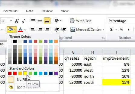
Microsoft Excel 2010 includes a specific tool that you can use to fill a selected cell with a certain color. You can even choose the color that you want to use to fill that cell. That tool is accessed by clicking the Home tab at the top of the Excel window, and is circled in the image below. For example, when I am creating a large spreadsheet, I like to use colors that are distinctly different but are not so distracting that the document becomes hard to read. If the text in your cells is black, then you will want to avoid using darker fill colors. Sticking to colors like yellow, light green, light blue, and orange will make it very easy for someone to recognize the different cells, but they will not have any difficulty reading the data within them. This is the most important part because the data is still the reason that the spreadsheet exists in the first place. To add color to the background of your cell, you must first click the cell to select it. Click the drop-down arrow to the right of the Fill color icon, then click the color that you want to apply to the selected cell. The background color will change to the color that you selected. If you want to know how to change fill color in Excel 2010, simply click the cell with the fill color that you want to change, then click the Fill color drop-down arrow and choose a different color. Now that you know how to color cells in Excel you can use this method to sort and organize your data by simply changing the color of the background in your spreadsheet cells. If you are not able to change the fill color using this method, then there is some other formatting rule applied to your cell that you need to adjust. Read this article to learn about removing conditional formatting from Excel.
How to Fill a Row With Color in Excel or How to Fill a Column With Color in Excel
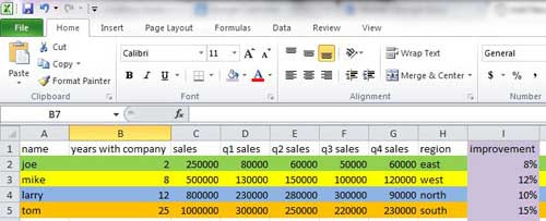
The process for applying color to a row or column in Excel is nearly the same as how to apply fill color in Excel to a single cell. Start by clicking the row or column label (either a letter or number) that you want to apply the fill color to. Once clicked, the entire row should be selected. Click the Fill color icon in the ribbon, then click the color that you want to apply to that row or column. Additionally, if you want to learn how to change the fill color in a row or column in Excel, simply select the filled column or row and use the Fill color icon to select a different color. By using these methods to apply fill colors to your Excel spreadsheet, you can make it much easier to see which row or column a particular cell is included within. The image below is an example of a spreadsheet that has been completely colored in, which should give you an idea of what you can do with this tool. Organizing data in this fashion is not particularly necessary when you are dealing with such a small amount of data but, for larger spreadsheets, it can make locating specific types of information much simpler. Note that using fill colors in this manner is best accomplished when you are done editing your data. The cell fill color won’t stick with the data if you start rearranging rows and columns, so you could wind up with a colorful mess. Fixing it is as easy as simply re-defining your fill colors, but that can be a pretty big waste of time if you have applied fill color to a lot of your data. One additional benefit to using fill colors in Excel is the ability to then sort based on those colors. Learn how to sort by fill color in Excel 2010 and take advantage of the formatting that you have applied to your cells. The next section provides additional information on how to color cells in Excel, such as how to use conditional formatting, and how to apply cell color to multiple cells at the same time.
More Information on How to Format Cells with Cell Color in Microsoft Excel Spreadsheets
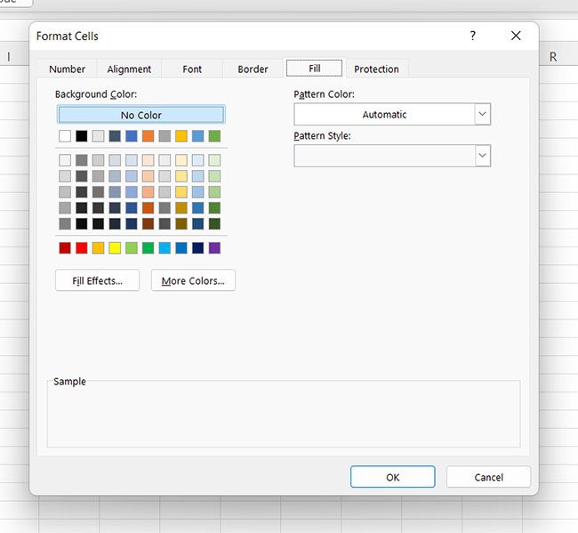
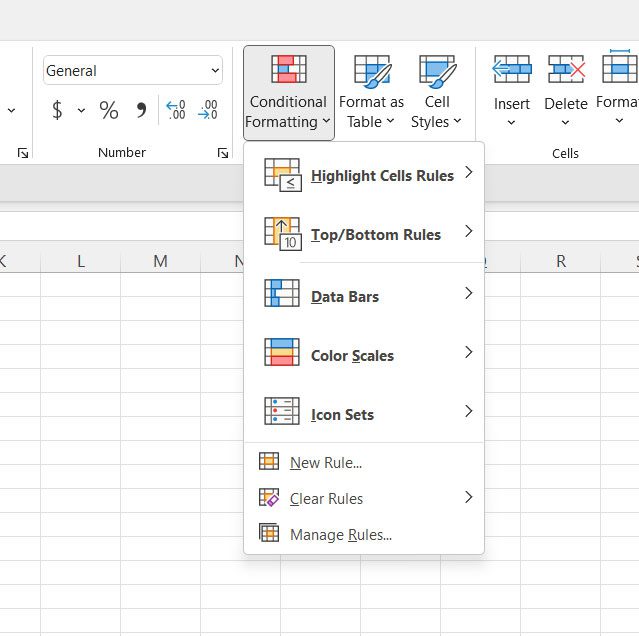
Note that you can apply cell colors to one cell, multiple cells, or you could even select the entire sheet by clicking on a single cell then pressing the Ctrl + A keyboard shortcut. There are some other ways that you can create colored cells in Excel. For example, if you select all the cells that you want to color, even if there are multiple cells, then you can right-click on those cells and choose the Format Cells option. This opens the Format Cells dialog box. Here you will find a Fill tab at the top of the window that you can use to change the cell background color. You can even click the More Colors button here if you would like to use a color code to modify the color of the cell. One other option that you can consider to highlight data with cell colors is to apply conditional formatting. This lets you choose a conditional format based on the cell value so that Excel will format only cells that fit those criteria. For example, you could choose to format cell values over zero with a green color and make a red cell if it contains a value below zero, or you could apply background colors based on the selected cells containing certain words. You can find the Conditional Formatting option on the Home tab in the Styles section of the ribbon. Simply click the Conditional Formatting button, choose the parameters, and select format options based on how you want excel to color in your cells. The rules applied during the process of setting up the conditional formatting parameters will apply the cell color based on the options you select. If none of the color code based options that you see on this dropdown menu offer the solution that you are looking for, then you could click the New rule button and choose your own format. If you are using Google Sheets and want to be able to color cells, then you are also able to do that. Simply open the spreadsheet in Google Sheets, select the cells that you wish to color, then click the Fill Color button in the toolbar above the spreadsheet. You could also click the Format button at the top of the window and use Conditional formatting or alternating colors there for some more advanced methods of coloring spreadsheet cells.
Additional Sources
After receiving his Bachelor’s and Master’s degrees in Computer Science he spent several years working in IT management for small businesses. However, he now works full time writing content online and creating websites. His main writing topics include iPhones, Microsoft Office, Google Apps, Android, and Photoshop, but he has also written about many other tech topics as well. Read his full bio here.
