It’s also prone to errors, so you might be looking for a better way to combine data that you currently have in separate cells in Excel. This guide is going to show you how to use the concatenate Excel formula to combine data from cells in your spreadsheet. The steps for the formula are addressed briefly at the start of this article, then we go into more depth with pictures below.
How to Use the Excel Concatenate Formula
Our tutorial continues below with additional information on using the Excel concatenate formula, including pictures of these steps. The examples in the table above provide a quick overview of what you could expect from a handful of concatenate variations where you have an A2 value of “John” and a B2 value of “Smith.” Microsoft Excel 2013 has a number of tools and features, like the subtraction formula in Excel, that can help you to increase your productivity, or minimize the amount of time that you need to spend doing data entry. One way in particular that you can take advantage of Excel’s formulas is with the CONCATENATE function. This allows you to combine data from two cells into one. So, for example, if you have a table of customer information that has first and last names separated into different cells, but you need to combine them into one cell for something else, then you can avoid a lot of tedious typing with the CONCATENATE ability. Our guide below will show you how to use it, as well as a couple of ways that you can modify it to add spacing or additional text to the existing data in your cells. It’s really a powerful and handy tool to be familiar with, and it can help to replace a lot of the more annoying or time-consuming Excel tasks that you might have had to perform in the past. Microsoft Excel formatting options can be a great way to fix display issues with your data. You can find out more about Excel formatting with our tutorial here.
How to Use Concatenate in Excel 2013 to Combine Data From Multiple Cells
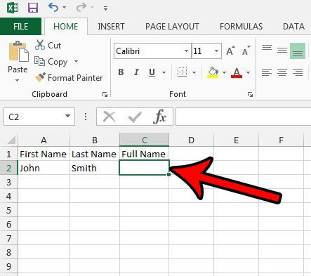
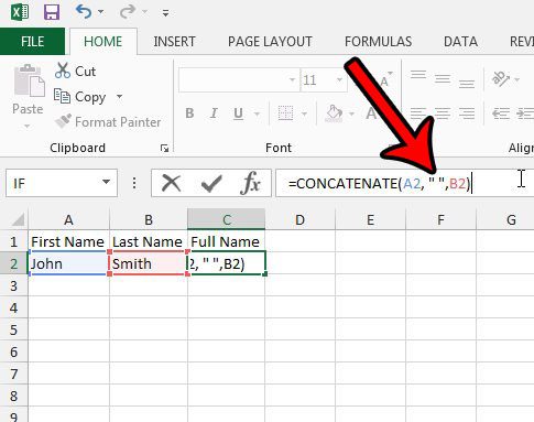
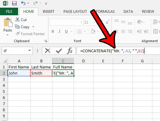
The steps in this article will show you how to use the CONCATENATE function to quickly combine data from two cells. Additionally you can use the CONCATENATE function to add text or numbers before or after a cell value. This is something I often use if I need to add the same text to a column of cells and want to avoid manually typing all of it. Step 1: Open your spreadsheet in Excel 2013. Step 2: Click inside the cell where you want to display the combined values. Step 3: Type =CONCATENATE(A2, B2) but replace the A2 part of the formula with the cell location for the first cell that you wish to combine, and replace B2 with the second cell. You can then press Enter on your keyboard to execute the formula. You may notice that Excel will combine exactly what is in those cells. In my example above, that formula would result in JohnSmith. Unfortunately that is not the desired outcome of this, so I need to make an adjustment to the formula. If I change the formula to =CONCATENATE(A2, " “, B2) then it will display the desired “John Smith” result. Note that there is a space between the quotation marks in that formula. Along those same lines, we can add text to this formula as well. By changing the formula to =CONCATENATE(“Mr. “, A2, " “, B2) we would have a resulting cell value of “Mr. John Smith.” The CONCATENATE formula is just one of many useful formulas in Excel. This article talks about customizing the VLOOKUP formula in Excel 2013, which is helpful when you want to use a value to find a related value.
Additional Sources
After receiving his Bachelor’s and Master’s degrees in Computer Science he spent several years working in IT management for small businesses. However, he now works full time writing content online and creating websites. His main writing topics include iPhones, Microsoft Office, Google Apps, Android, and Photoshop, but he has also written about many other tech topics as well. Read his full bio here.


