If you have used formulas before, then the Max function should be relatively familiar. If not, then you should read our article about Excel 2013 formulas. But if you just need to know how to determine the highest value in a range of cells, follow our guide below.
Using the Max Function in Microsoft Excel 2013
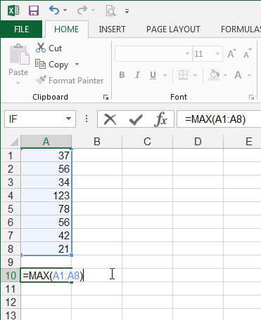
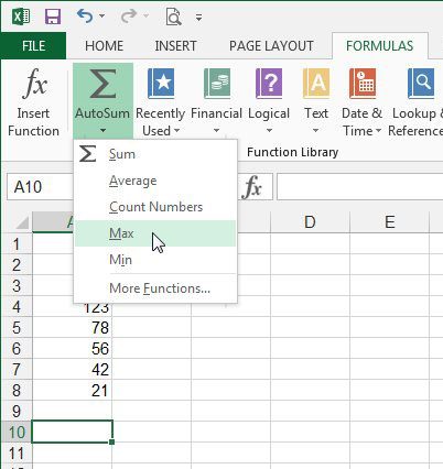
The steps in this article will show you how to find the highest value among a group of consecutive cells that you select from one of the columns in your spreadsheet. Once you enter the formula that we will be defining, the highest value will be displayed in the cell that you select. If you want to use some other formulas, then our article about how to subtract in Excel can show you a really useful one. Step 1: Open your spreadsheet in Microsoft Excel 2013. Step 2: Click inside the cell where you want to display the highest value. Step 3: Type =MAX(XX:YY), where XX is the first cell in the range of cells that you are comparing, and YY is the last cell in the range. Press Enter on your keyboard after you have finished entering the formula. In my example image below, the first cell is A1 and the last cell is A8. Rather than manually typing the formula, you can also select it by clicking the Formulas tab, clicking AutoSum, then clicking Max. Would you also like to learn how to find the average value in a range of cells? This article will show you the process.
Additional Sources
After receiving his Bachelor’s and Master’s degrees in Computer Science he spent several years working in IT management for small businesses. However, he now works full time writing content online and creating websites. His main writing topics include iPhones, Microsoft Office, Google Apps, Android, and Photoshop, but he has also written about many other tech topics as well. Read his full bio here.
You may opt out at any time. Read our Privacy Policy