How to Hide a Row from View in Excel 2010
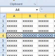
Note that this method is used only to hide the rows from view. They are still technically there, and any formulas that use data from the hidden row will still be calculated. The purpose of hiding rows is to filter down visible data so that you are only seeing what you need to see, but keeping the data accessible should you need to return it to view at a later point in time. With that in mind, follow the tutorial below to learn how to hide a row in Excel 2010. Step 1: Open the spreadsheet containing the row that you want to hide. Step 2: Click the row number at the left side of the window for the row that you want to hide.
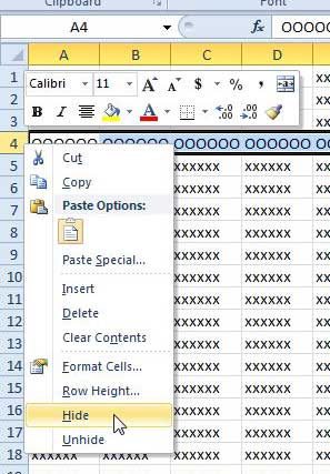
Step 3: Right-click the selected row number, then click the Hide option.
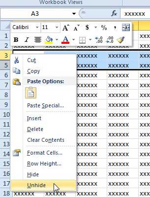
You will notice that the row numbers at the left side of the window will now skip the row that you just hid. You can unhide hidden rows by selecting the rows around the hidden row, then clicking the Unhide option.
This same method will work for multiple rows, as well. Simply select the rows that you want to hide instead of selecting a single row, then perform the steps above. We have also written about how to hide columns in Excel 2010, which is a very similar process. You can also hide row and column heading in Excel 2010, if you wish. After receiving his Bachelor’s and Master’s degrees in Computer Science he spent several years working in IT management for small businesses. However, he now works full time writing content online and creating websites. His main writing topics include iPhones, Microsoft Office, Google Apps, Android, and Photoshop, but he has also written about many other tech topics as well. Read his full bio here.
You may opt out at any time. Read our Privacy Policy