You’ve probably done things like bold text or underline text in the past, but there is another type of styling called “strikethrough” that draws a horizontal line through the text. If you see some of this in your spreadsheet and would like to remove it, then our tutorial below on how to remove strikethrough in Excel will show you how.
How to Remove Microsoft Excel Strikethrough Formatting
Our guide continues below with additional information on how to remove strikethrough in an excel spreadsheet, including pictures of these steps. Text formatting effects like bold, italic, and underline can be useful when displaying data in Excel. Excel even offers formatting options when you need to specify that data is numeric rather than text. But if some of your data has a line through it, then you may be looking for a way to remove strikethrough in Excel. Most applications where you can write something will have ways for you to format text. Most Microsoft Office applications like Word or Outlook have a number of options. The strikethrough effect in Microsoft Excel 2010 is helpful when you wish to indicate that information in a cell should be ignored, yet you do not want to delete that information. But the strikethrough effect can be distracting, especially when it is used a lot, and the effect remains applied to the information if you copy and paste it into another spreadsheet or document. If you are finding the strikethrough effect to be problematic, then you are probably looking for a way to remove it. The effect is not included in the ribbon, however, so you need to use a keyboard shortcut or a secondary menu in order to apply or remove it. Our tutorial below will show you where to find the strikethrough option so that you can eliminate it from your selected cells.
How to Remove the Line Through Text in Excel 2010 (Guide with Pictures)
The steps in this article will assume that you have a spreadsheet which contains text with the strikethrough effect, and that you wish to remove that effect. If you instead wish to add the strikethrough effect to some of the cells in your spreadsheet, the this article will show you how.
Step 1: Open your spreadsheet in Microsoft Excel 2010.
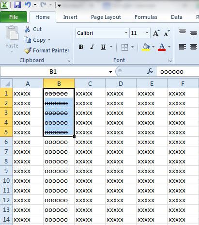
Step 2: Select the cell(s) containing the strikethrough text that you wish to remove.
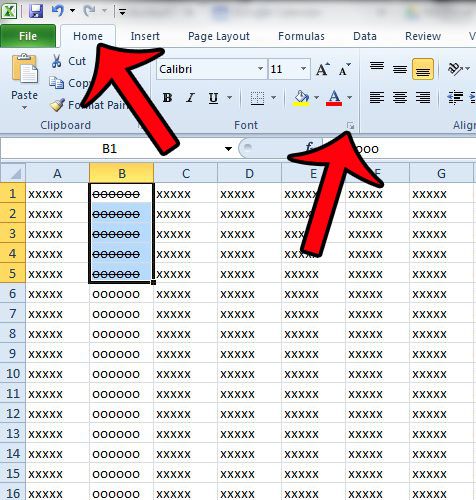
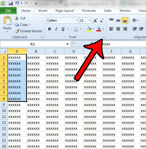
Step 3: Click the Home tab at the top of the window, then click the Format Cells: Font button at the bottom-right corner of the Font section in the Office ribbon.
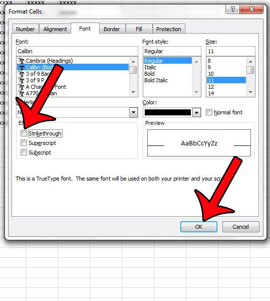
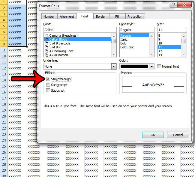
Step 4: Check the box to the left of Strikethrough, then click the OK button at the bottom of the window.
The method for adding strikethrough to text in Excel 2010 is very similar. The steps below will walk you through it.
How to Strikethrough in Excel 2010
The steps below will show you how to select a group of cells and apply the strikethrough effect to the data in those cells.
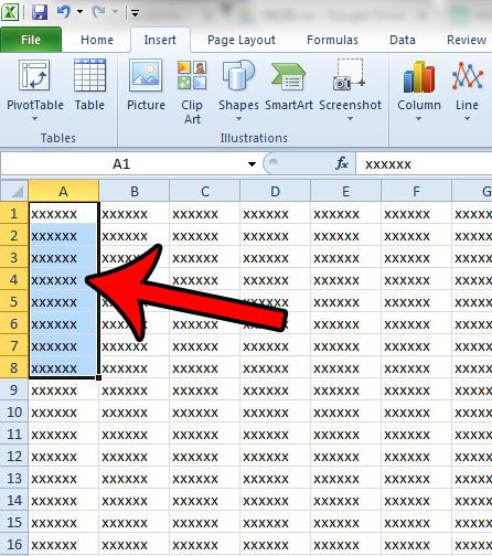
Step 1: Use your mouse to highlight the Excel cells that you would like to strikethrough.
Step 2: Click the Home tab at the top of the window.
Step 3: Click the small dialog launcher button at the bottom-right corner of the Font ribbon section.
Step 4: Check the box to the left of Strikethrough to apply the effect to the data in the selected cells. Click the OK button to close the window.
Note that you can also toggle the strikethrough effect on or off for selected cells by using the default shortcut. The shortcut for the strikethrough effect in Excel 2010 is Ctrl + 5. is there too much formatting applied to your cells, and you would prefer to remove all of it at once? Learn how to clear cell formatting in Excel 2010 from a group of cells, or even the entire spreadsheet. After receiving his Bachelor’s and Master’s degrees in Computer Science he spent several years working in IT management for small businesses. However, he now works full time writing content online and creating websites. His main writing topics include iPhones, Microsoft Office, Google Apps, Android, and Photoshop, but he has also written about many other tech topics as well. Read his full bio here.
