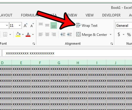
This happens when there are more characters in the cell that can fit within the visible cell boundaries. While you might have tried adjusting the row height and column width before, another option would be to wrap the text in the cells. Our tutorial below will show you how to wrap text in Microsoft Excel using a button found on the Home tab.
How to Change the Wrap Text Setting in Excel
Our guide continues below with additional information on how to wrap text in every cell in an Excel spreadsheet, including pictures of these steps. Microsoft Excel provides you with a lot of tools that let you control the width of your columns and the height of your rows. We’ve written about how to expand cells in Excel as a means to make this a little easier, but that might not provide you with the results that you needed. You may have already found the option to wrap text in Excel 2013, but you might have noticed that it will only apply to the cell that is currently selected. This is not something that can only be done to one cell at a time, however. You can wrap text for multiple cells at once if they are all selected, and you can even wrap text for every cell in a spreadsheet in Excel 2013. Our guide below will show you how to select all of your cells, then apply the “Wrap Text” effect to those selected cells. Your cells will then automatically resize to display the data contained within them. You can read our how to wrap text in Google Sheets tutorial if you also use Google’s spreadsheet application and need to perform this action there as well.
How to Apply Wrap Text to an Entire Spreadsheet in Excel 2013 (Guide with Pictures)
The steps below are going to show you how to select your entire spreadsheet, then apply the Wrap Text formatting to that spreadsheet. Wrap Text will automatically force your data onto additional lines so that it remains visible within the current confines of your column widths. The height of your cells, however, will change to accommodate the increased number of lines within the cells.
Step 1: Open your spreadsheet in Excel 2013.
Step 2: Click the button above the Row 1 heading and to the left of the Column A heading to select the entire worksheet.
You can also select the entire spreadsheet by clicking on any cell, then pressing Ctrl + A on your keyboard.
Step 3: Click the Home tab at the top of the window.
Step 4: Click the Wrap Text button in the Alignment section of the ribbon.
Note that you can manually add additional lines inside a cell by clicking at the point in the cell where you want the line break, then holding down the Alt key on your keyboard and pressing Enter. You can perform a similar function by autofitting the column widths in Excel 2013. This will automatically expand the width of the columns to display the data contained within them.
Keep Reading
After receiving his Bachelor’s and Master’s degrees in Computer Science he spent several years working in IT management for small businesses. However, he now works full time writing content online and creating websites. His main writing topics include iPhones, Microsoft Office, Google Apps, Android, and Photoshop, but he has also written about many other tech topics as well. Read his full bio here.
You may opt out at any time. Read our Privacy Policy


