While you might have tried ot resize the cell or manually insert line breaks, you can also use an option that will cause the text to “wrap.” Our guide below will show you how to wrap text in Google Sheets so that you can more easily view the data that you are working with.
How to Use the Google Sheets “Wrap Text” Option
Our tutorial continues below with additional information on how to wrap text in Google Sheets, including pictures for the steps shown above. If you want to wrap text in Google Sheets mobile, click here to jump to that section of this article. Click on any of the links in the table of contents above to jump to that section in the article, or continue scrolling down to read everything. Learning how to wrap text in Google Sheets is beneficial when you have a lot of text to display in a single cell that you need to be visible. We don’t always think about text formatting in Google Sheets and tend to compartmentalize them with documents, as options like line spacing in Google Docs don’t often present themselves in the cells of a spreadsheet. When you type a lot of data into a cell in your Google Sheets spreadsheet, one of several things can happen. The text can overflow into the next cell if it’s empty, it can be forced to another line within the cell, or it can be clipped so that only the text that fits in the cell is visible. Depending on your preferences, it’s possible that your spreadsheet cells are behaving differently than you would like in this regard. Fortunately, this is something that you can adjust so that your text wrapping behaves how you want. Our article below will show you how to make that adjustment. Microsoft Excel spreadsheets with a lot of links can be tough to work with. You can read our break links in Excel article and find out how ot get rid of those links quickly.
How to Change Text Wrapping Setting in Google Sheets (Guide with Pictures)
The steps in this guide were performed in the desktop version of the Google Chrome web browser but will work in other desktop browsers like Safari or Edge as well. Now that you know how to wrap text in Google Sheets you will be able to use this option whenever you need to adjust the layout of the data in some of the cells in your spreadsheet. If you select multiple adjacent cells then the wrapped text setting you choose will apply to all of them. The next section explains more about the different text wrapping settings, including examples of each option.
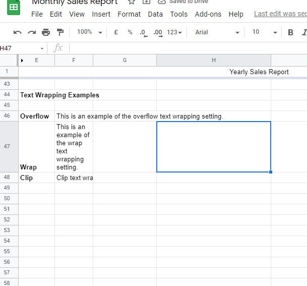
Examples of Google Sheets Text Wrapping Options
The text-wrapping settings in Google Sheets are:
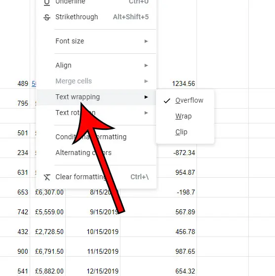
Overflow – text will display in the current cell and the next cell if it’s empty Wrap – text will be forced to additional lines within the current boundaries of the cell. This can adjust the height of the row automatically. Clip – the clip option only shows the text that is visible within the current boundaries of the cell. Note that the text is still in the cell, it’s just not visible.
You can select more than one cell in Google Sheets by clicking a row number to select the entire row, clicking a column letter to select the entire column, holding down the Ctrl key to click multiple cells, or clicking the gray cell above the row 1 heading. Now that you know how to wrap text in Google Sheets and use one of the different available options, you can read about another way that you can format text wrapping in a Google worksheet.
Another Way to Perform Google Sheets Text Wrapping
There is another method that you can use if you find the Text wrapping button to be difficult to identify, or if you prefer to use the top menu. Step 1: Select the cells that you wish to modify.
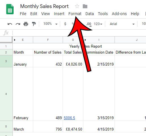
Step 2: Click the Format tab at the top of the window. Step 3: Choose the “Text wrapping” option, then select the style of text wrapping to apply to the selected cells.
How to Apply a Text Wrap Setting in Google Sheets Mobile
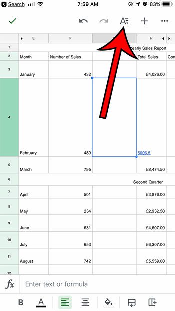
A final way that you can wrap the text in Google Sheets cells involves the mobile app. If you use the Google Sheets app then you may have been searching for the Wrap Text icon so that you didn’t need to make this change in Google Sheets manually. Luckily you can do most of the things that you need to edit your Google Sheet in the app, and it starts by using the Formatting button that Google Sheets offers on iOS and Android devices. Step 1: Open the Sheets app, then open the file containing the cells to modify.
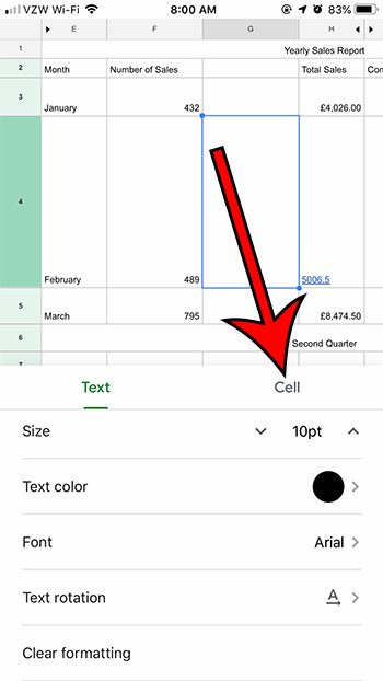
Step 2: Tap on the cell to adjust, then tap on the “Format” button. Step 3: Choose the “Cell” tab at the top of the menu. Step 4: Tap the button to the right of “Wrap text” to turn it on. If you are adjusting the text wrapping settings for your cells, then you may also want to consider adjusting the cell alignment. We continue below with information on that as well.
How to Change Vertical Alignment in Google Sheets
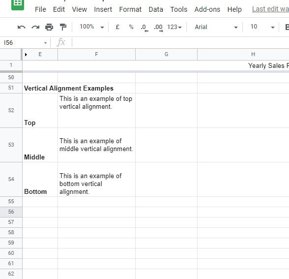
The vertical alignment of your cell data affects where in the cell the data is displayed. By default, cell data is aligned to the bottom of the cell in Google Sheets. You have the option of aligning your data to the top, middle, or bottom of the cell. There is a Vertical align button in the toolbar above the spreadsheet where you can set the vertical alignment for your selected cell(s.) You can also access vertical alignment options by going to Format > Align > and choosing an option there. Examples of these vertical alignment options are shown below. You can also elect to change the horizontal alignment by following the steps in the next section.
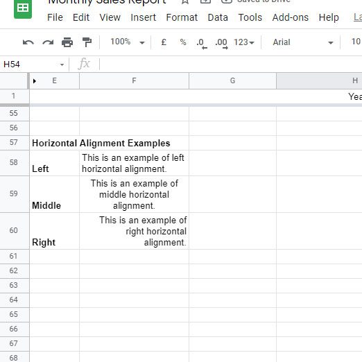
How to Change Horizontal Alignment in Google Sheets
While the options in the section above concern the vertical alignment of your cell data, you can also choose how your data is aligned horizontally in your cells. By default cell data is aligned to the left in Google Sheets. The available horizontal alignment options include left, middle, and right. There is a Horizontal align button in the toolbar above the spreadsheet where you can select the desired horizontal alignment for your selected cell or cells. You can also find horizontal alignment options by clicking Format > Align > and choosing an option from the menu there. Examples of Google Sheets horizontal alignment are shown below. The text wrapping setting that you apply to your cell(s) won’t affect the actual data contained within those cells. This only changes the way that the text is shown in the cells. If you were to copy data from a cell with text wrapping, for example, then any visual line break wouldn’t be included when pasting that data into another cell or application. If you have the desired wrap setting and it still doesn’t look right, you could try changing the column width as well. You can do this by clicking on the right border of any of your column headers and dragging it left to make it smaller, or dragging it right to make it larger. You can do the same thing with the borders by your row headers to change the height of your cells. Is there a lot of formatting in your spreadsheet that’s difficult to fix by looking for each individual setting? Find out how to clear formatting in Google Sheets and expedite that process.
Related Guides
How to merge cells in Google Sheets How to alphabetize in Google Sheets How to subtract in Google Sheets How to change row height in Google Sheets
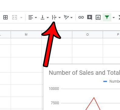
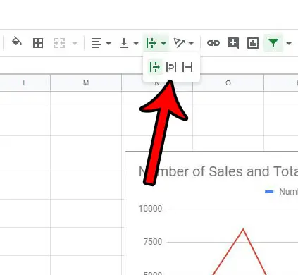
Next, you will click the “Text wrapping” button in the toolbar and select from one of the wrap options found there. These options are “Overflow,” “Wrap,” and “Clip.” In Google Sheets you can select the cell that you would like to change, then hold down the Alt key, press O to expand the Format menu, press W to expand the Text wrapping menu, then press O for Overflow, W for Wrap, or C for Clip. – Google Sheets overflow keyboard shortcut – hold Alt, press O, then W, then O– Google Sheets wrap keyboard shortcut – hold Alt, press O, then W, then W– Google Sheets clip keyboard shortcut – hold Alt, press O, then W, then C If you don’t want to use this shortcut, you will need to use either the option from the “Format” tab in the menu, or the “Text wrapping” button in the toolbar above the spreadsheet. If you go to the Format menu, select Text wrapping from the drop down menu, then select Wrap, Overflow, or Clip. Additionally, you may want to check that there aren’t any line breaks or spaces in the cell text, as that can affect the way that text wrapping looks as well. Assuming that there is no other formatting setting that is affecting the contents of your cell, then that text should wrap as expected when you choose the “Wrap” option. In Google Docs it refers to the way that your document interacts with an image in the document. You can adjust Google Docs text wrapping by right-clicking on the image and selecting the “Image options” button. Next, select the “Text wrapping” tab at the left side of the window, then choose the way that you want your content to wrap around the picture. The options in Google Docs are “Inline with text,” “Wrap text,” and “Break text.” After receiving his Bachelor’s and Master’s degrees in Computer Science he spent several years working in IT management for small businesses. However, he now works full time writing content online and creating websites. His main writing topics include iPhones, Microsoft Office, Google Apps, Android, and Photoshop, but he has also written about many other tech topics as well. Read his full bio here.
You may opt out at any time. Read our Privacy Policy