Fortunately it is possible to unhide these rows so that you can view and edit the information contained within them. Our guide below will show you how.
How to Show Missing Rows in Excel 2013
The steps below are going to show you how to unhide all of the hidden rows in Excel 2013. Often times rows are hidden for a good reason, and you may find that displaying the hidden rows makes the spreadsheet difficult to read. You can read this article to learn how to hide rows in Excel 2013. Step 1: Open the spreadsheet with the hidden rows in Excel 2013. Step 2: Click the cell at the top-left corner of the spreadsheet, between the 1 and the A. This is going to select the entire worksheet.
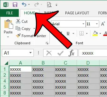
Step 3: Click the Home tab at the top of the window.
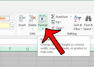
Step 4: Click the Format button in the Cells section of the ribbon at the top of the window.
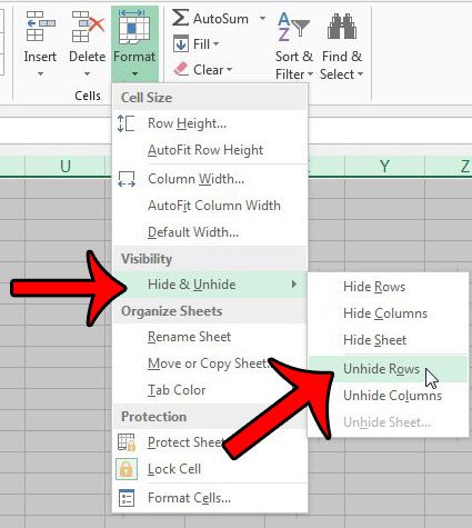
Step 5: Click the Hide & Unhide option, then click Unhide Rows.
Are you running into problems with multi-page Excel spreadsheets that are hard to read when they are printed? Print the header row on every page and make it easier to associate cells with their appropriate columns. After receiving his Bachelor’s and Master’s degrees in Computer Science he spent several years working in IT management for small businesses. However, he now works full time writing content online and creating websites. His main writing topics include iPhones, Microsoft Office, Google Apps, Android, and Photoshop, but he has also written about many other tech topics as well. Read his full bio here.